What I Learned Forecasting Pharmacy Sales and Why the Simplest Model Won

I spent a good chunk of this project convinced that more sophistication would win; more features, more models, more tuning. It didn't. The model that beat nine competitors, including XGBoost, LightGBM, and a tuned Prophet, LightGBM ensemble, was a plain linear regression. Here's how I got there, what the data taught me along the way, and why the "boring" answer turned out to be the right one.

(Try the interactive predictor to see the winning model's forecasts against real, held-out sales data.)

Why this matters

Pharmacies live and die by getting demand forecasts right in both directions. Overstock a drug with a short shelf life and you're writing off expired inventory. Understock it during a demand spike and a patient can't get medication they need. That asymmetry , get it wrong high, lose money; get it wrong low, risk patient access , shaped almost every decision in this project, right down to which error metrics I trusted.

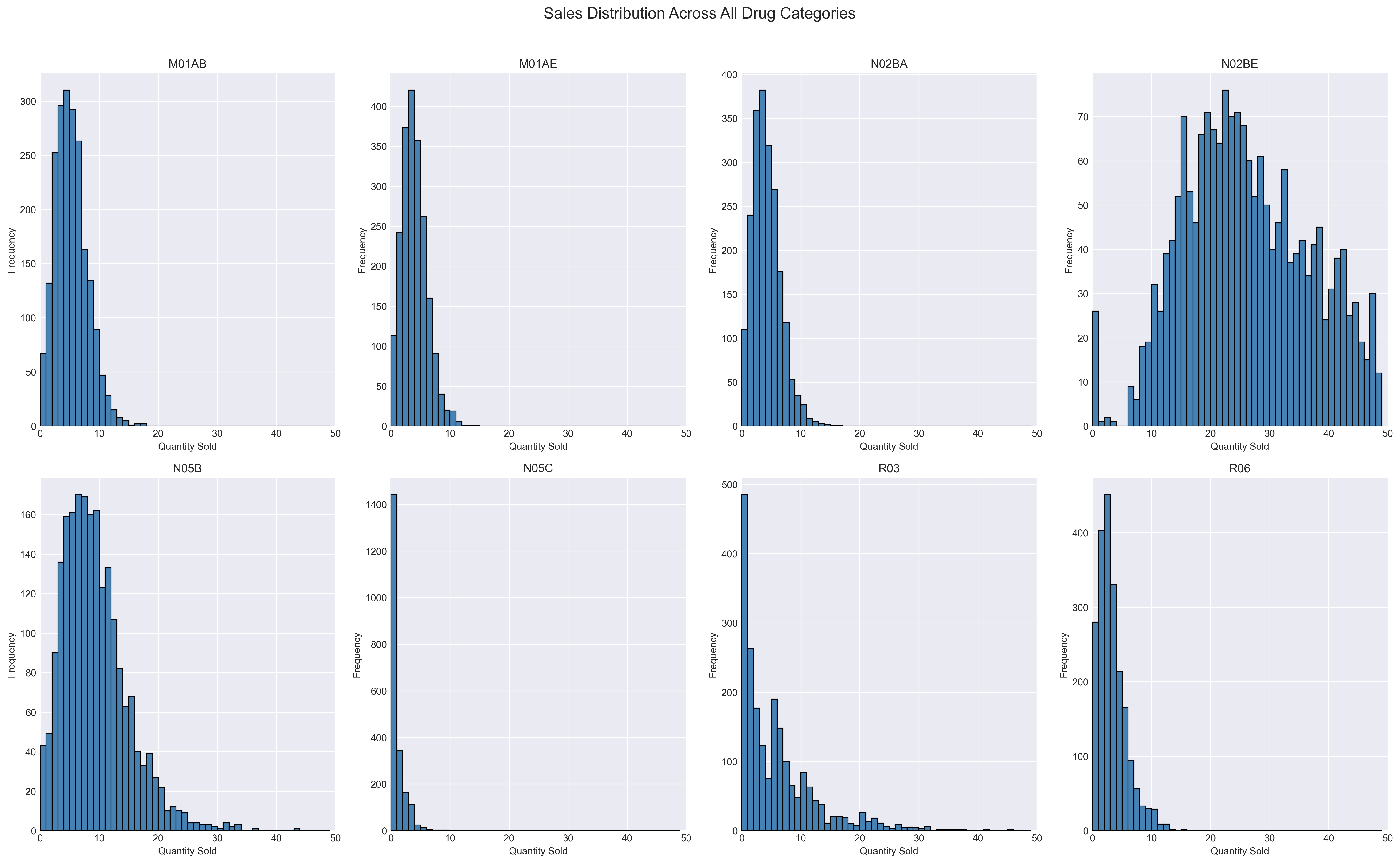
I worked with six years (2014–2019) of daily sales data from a single pharmacy, covering eight drug categories. I chose to go deep on one category first; R03, drugs for obstructive airway diseases, rather than spreading thin across all eight, on the hypothesis that respiratory drug demand would show a strong, learnable seasonal signal tied to cold and flu season.

What the data actually looked like

Before touching a model, I spent time just looking. A few things stood out:

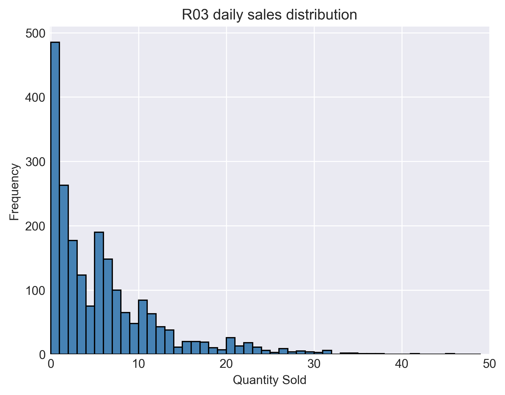
R03 sales are mostly zero. Out of roughly 2,100 days, 484 had zero R03 sales. That's not missing data. Pharmacies genuinely don't sell every drug category every day, but it meant standard regression metrics like R² were going to look ugly no matter what, since R² punishes variance around a mean that's dragged toward zero by intermittent demand.

26 days were undocumented closures, not real zero-demand days. Sundays accounted for most of the zero-sales pattern, but a smaller cluster of dates - New Year's Day, a suspicious recurring July 7th, a pre-Christmas date - looked like the pharmacy simply wasn't open. I interpolated across those so the model wouldn't learn "this specific calendar date always means zero" when the truth was "the doors were closed."

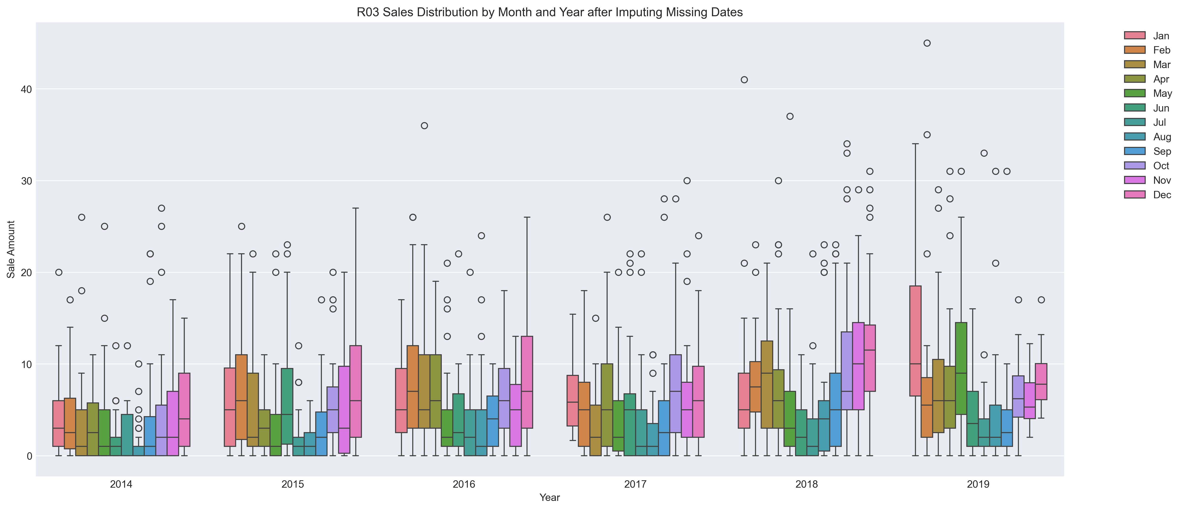
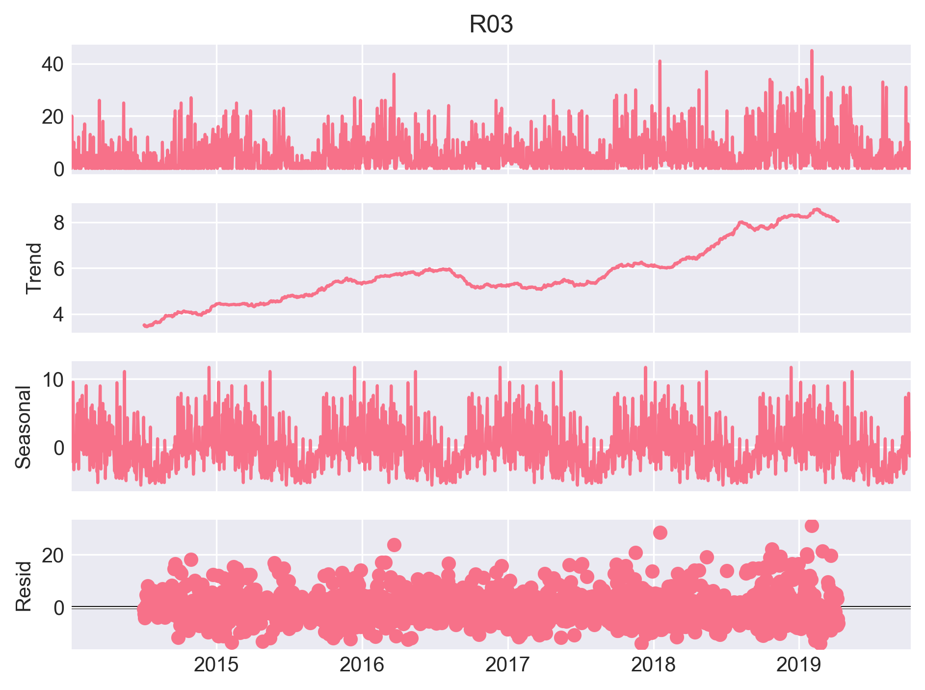
Seasonality was real, but not where I first guessed. My initial hypothesis was that R03 would peak in winter and spring. The actual pattern, confirmed by a seasonal decomposition and corroborated by monthly boxplots, was sharper: demand climbs from November through February, holds moderate into April, drops hard through the summer, and recovers toward year-end. December and February had the highest median sales; July and August the lowest. I rewrote the hypothesis to match the evidence rather than forcing the evidence to match my first guess.

Seasonal Decomposition of R03 sales

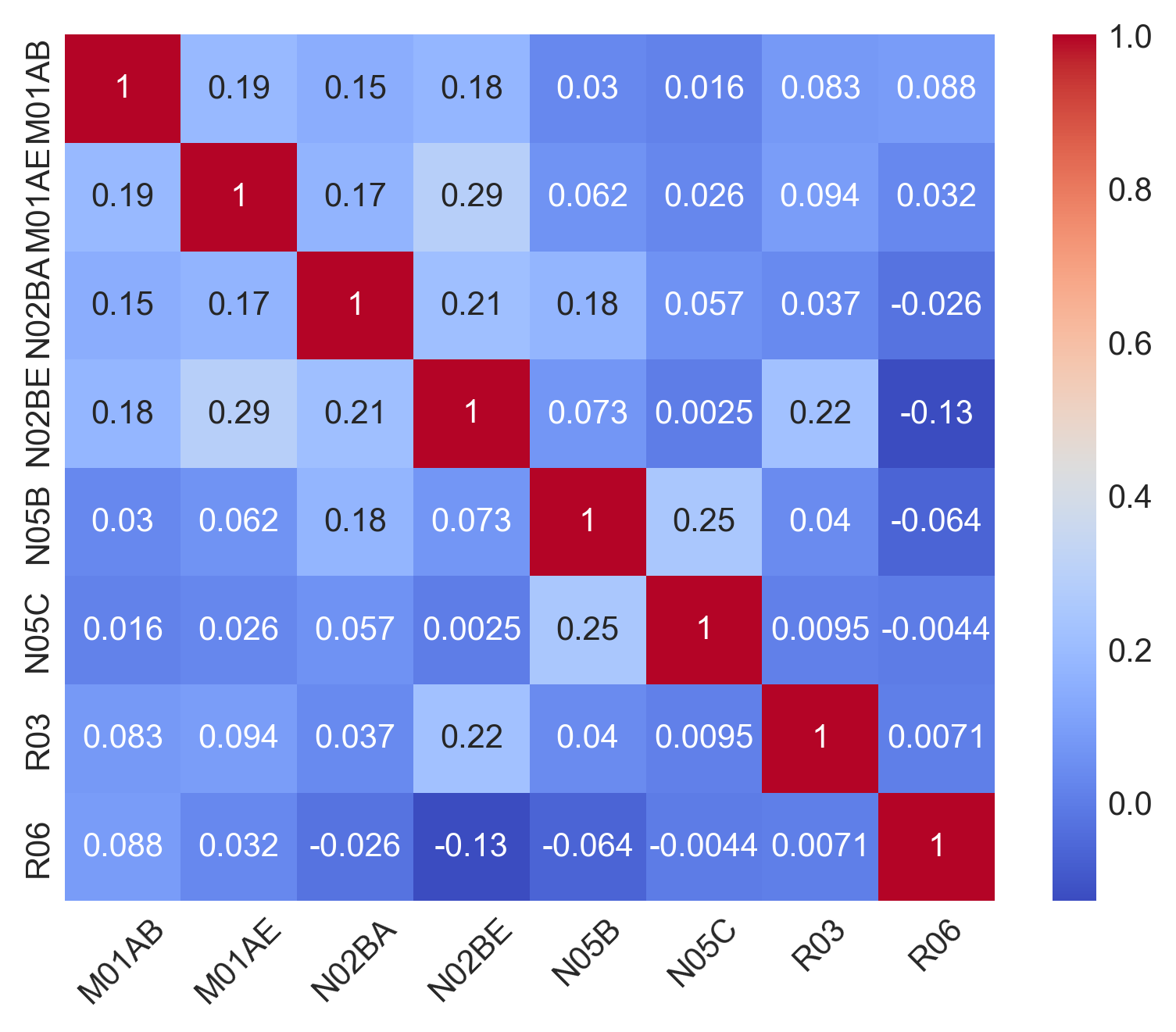
R03 and R06 (antihistamines) were essentially uncorrelated (0.007). I'd expected some overlap since both are respiratory-adjacent, but they're driven by opposite seasons; R06 by spring/summer pollen, R03 by winter cold and flu. It was a useful reminder that "same general category" doesn't mean "same demand driver."

Turning insight into features , and getting it wrong first

My first modeling attempt was a disaster, and a useful one. That first linear regression scored an R² of ,0.94 , worse than just predicting the mean every day. The autopsy turned up a chain of avoidable mistakes:

• One-hot encoding all four seasons created perfect multicollinearity (they always summed to 1), and I'd also fed the model both Month and Season, which encode almost the same information twice.
• The model only had a 52-week lag feature, meaning it only "remembered" what happened a year ago, with no sense of last week's momentum or this week's trend.
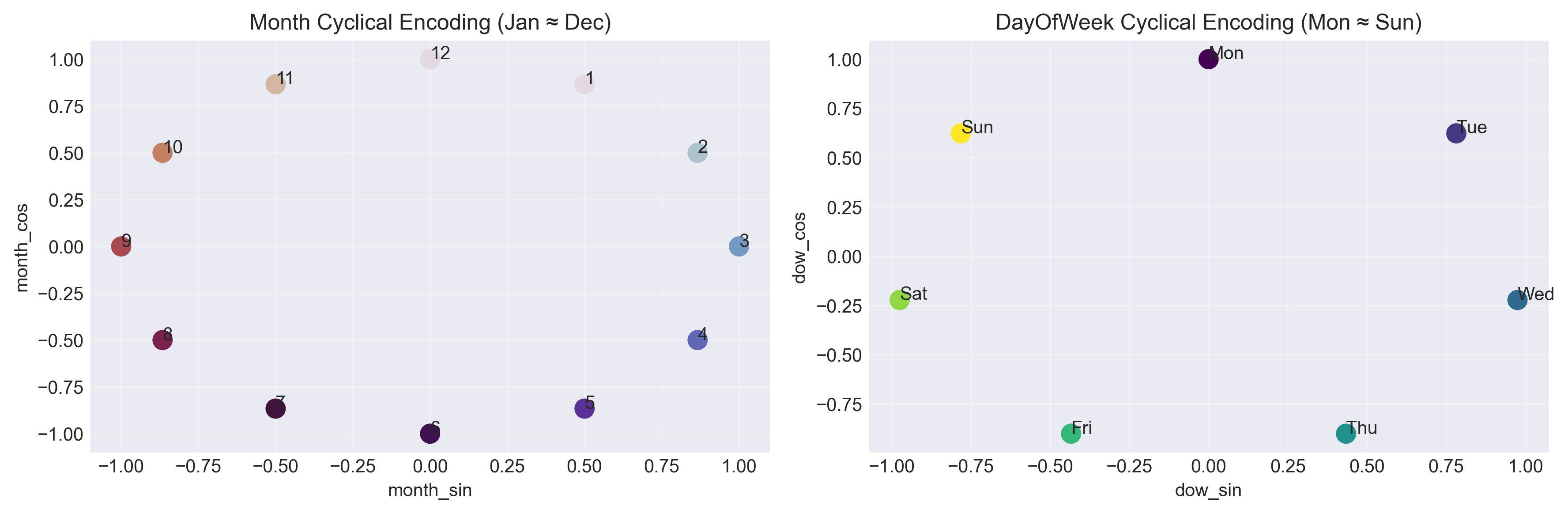
• Month was encoded as a raw number 1–12, which tells a linear model that December (12) is numerically as far from January (1) as it is from a February that's actually right next door on the calendar.

The fix was to rebuild the feature set properly: multiple lag windows (1, 7, 14, 28, 52 days) so the model could see short, medium, and long-term memory; rolling means and volatility (shifted to avoid leaking the future into the past); cyclical sine/cosine encoding for month and weekday so the calendar wraps around correctly; and interaction terms for things like winter weekends, where I expected, and later confirmed, unusually high demand.

Picking a yardstick that actually matches the stakes

This is the part of the project I'd point to as most directly shaped by the "why this matters" framing above. Standard ML metrics (RMSE, MAE, R²) are built for well-behaved, continuous data. R03 is neither continuous (484 zero days) nor symmetric in what an error costs.

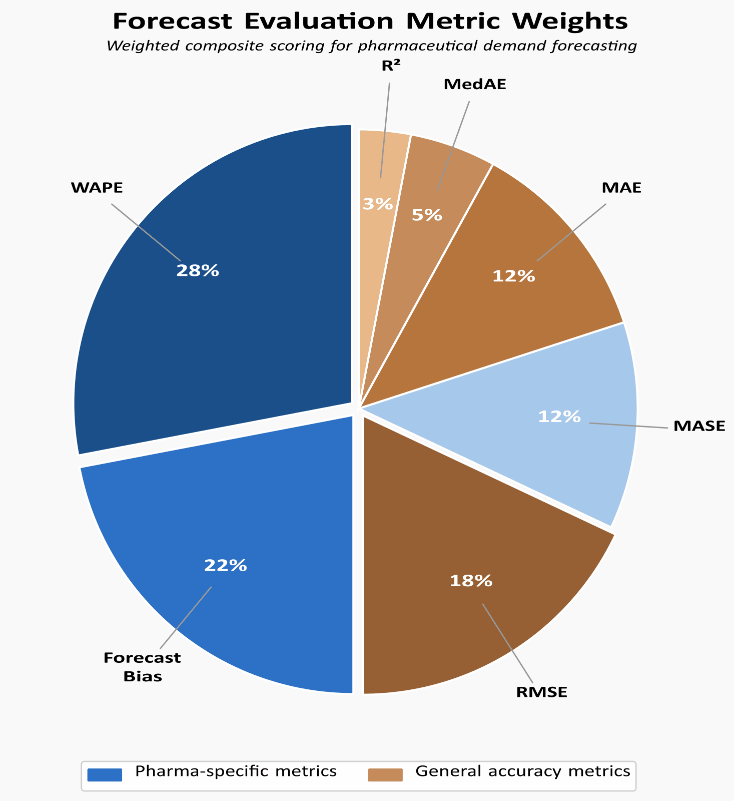
So, I leaned on pharmaceutical-specific metrics alongside the standard ones:

• WAPE (volume-weighted percentage error), which naturally down-weights the zero-sales days that would otherwise dominate a plain average.
• Forecast bias, split by direction , because for R03 specifically, underprediction (stockouts during flu season) is a patient-safety issue, while overprediction (waste) is "just" a budget line.
• MASE, to keep every model honest against the simplest possible baseline: yesterday's sales.

I ended up weighting pharmaceutical metrics at 62% of the final model ranking and general ML metrics at 38%, WAPE and bias carried the most weight, R² the least, since I knew going in it would look mediocre regardless of model quality.

The nine-model bake-off

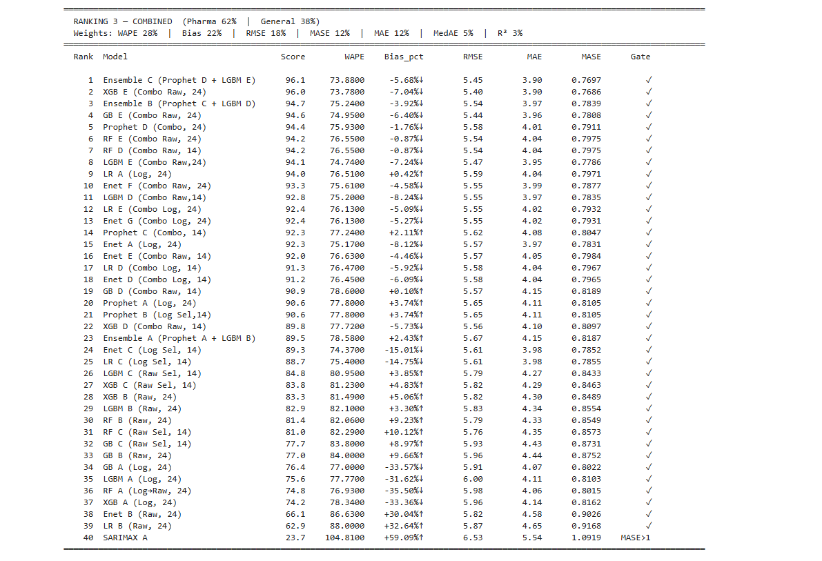
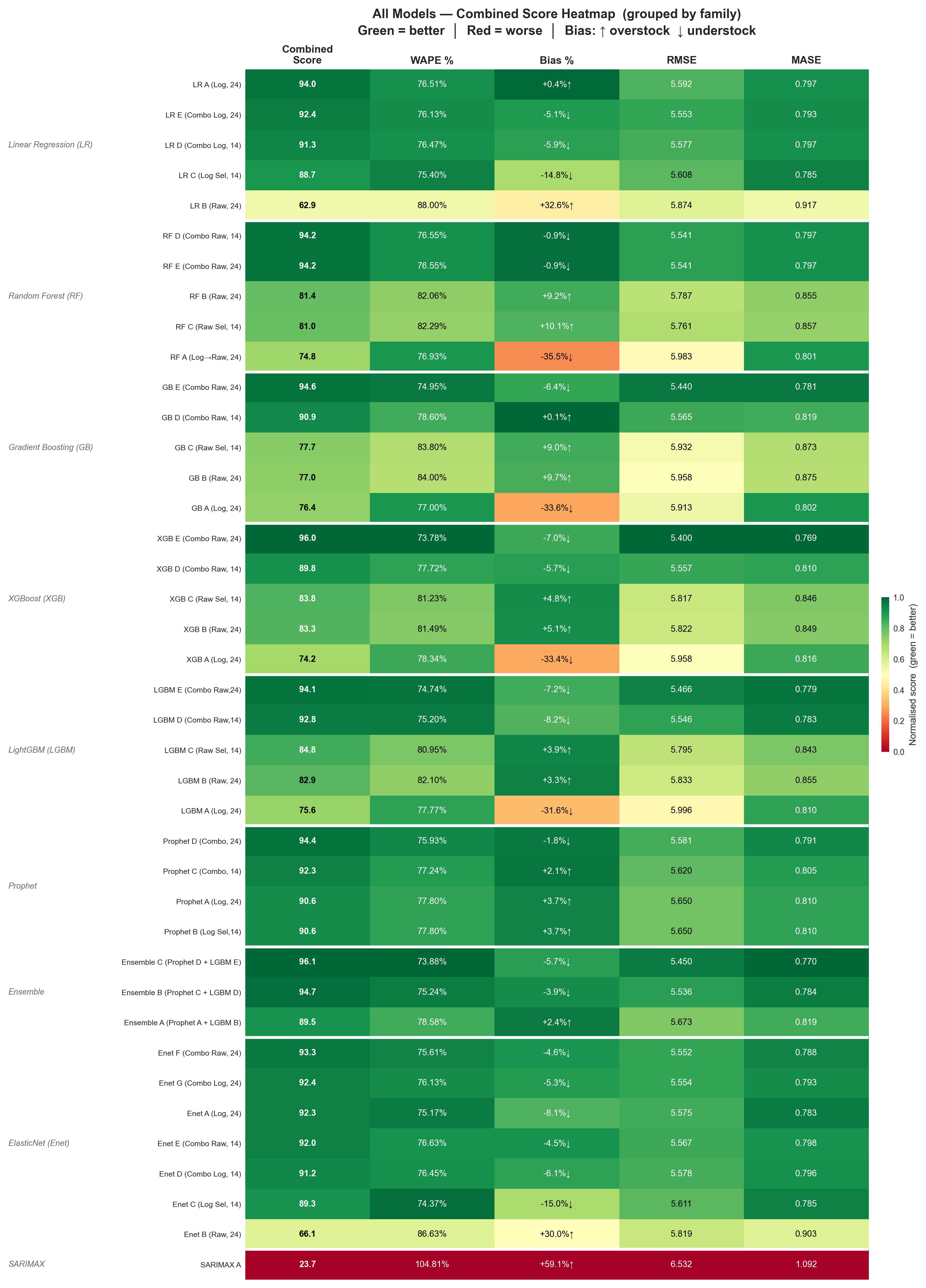
I trained and compared linear regression, ridge/elastic net, random forest, gradient boosting, XGBoost, LightGBM, Prophet, a Prophet+LightGBM ensemble, and SARIMA. A few findings held up across the board:

• Log-transforming the target helped linear models and hurt tree models. Every linear/regularized model improved with a log transform; every tree-based model performed better on raw data, since trees split on thresholds rather than fitting a line and don't need the distribution reshaped.
• All models beat the naive "yesterday's sales" baseline, narrowly. MASE scores clustered between 0.78 and 0.86, meaning the best models were only modestly better than doing nothing clever at all. That narrow spread told me feature engineering, not model sophistication, was where the real leverage was.
• SARIMA was the clear loser, and for a structural reason rather than a tuning one: it assumes a stationary, continuous series, and R03 is neither, it trends upward over the years and has hundreds of zero-demand days. A 19-hour training run wasn't enough to fix a fundamentally mismatched model.
• Elastic Net and plain linear regression were the strongest general-metrics performers, with the best WAPE, MASE, and near-zero forecast bias.

Hyperparameter tuning: the humbling part

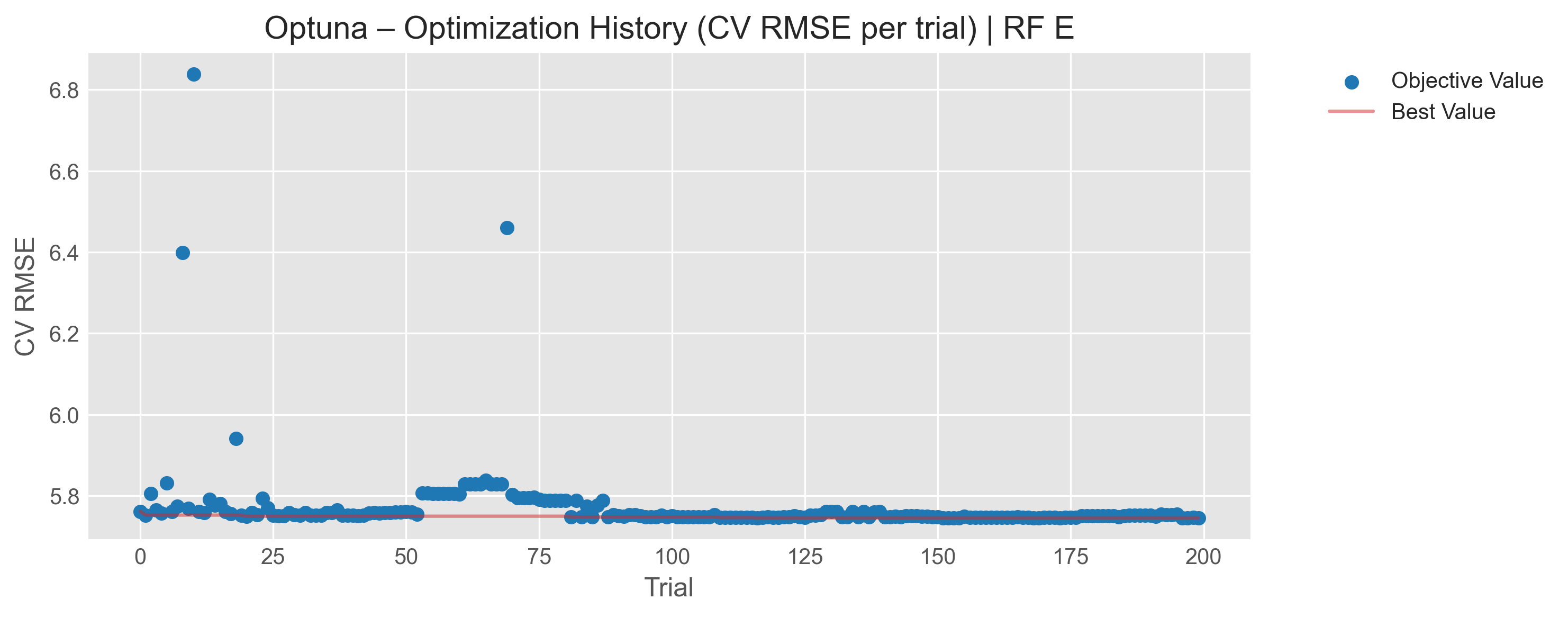
I ran 200-trial Bayesian searches (Optuna) on the top tree models and a grid search on Prophet, expecting tuning to meaningfully close the gap with the linear models. It mostly didn't. Tuned XGBoost, gradient boosting, and random forest all performed worse on the validation set than their untuned defaults, better on cross-validation, worse on the actual holdout. Tuned random forest was the most concerning case: it went from a near-neutral - 0.87% forecast bias to 8.46% - meaning tuning quietly introduced a systematic tendency to underpredict, exactly the failure mode that matters most for a drug like this. LightGBM and the Prophet+LightGBM ensemble were the only models where tuning was close to a wash rather than a regression.

I also tested a two-stage approach, first classify "will this week have sales at all," then regress on the non-zero weeks, on the theory that separating the zero-inflation problem from the regression problem might help. It didn't: the classifier was barely better than guessing on the non-zero/zero split, so I dropped the approach rather than build further complexity on a shaky foundation.

The twist: why the simplest model won on the real test set

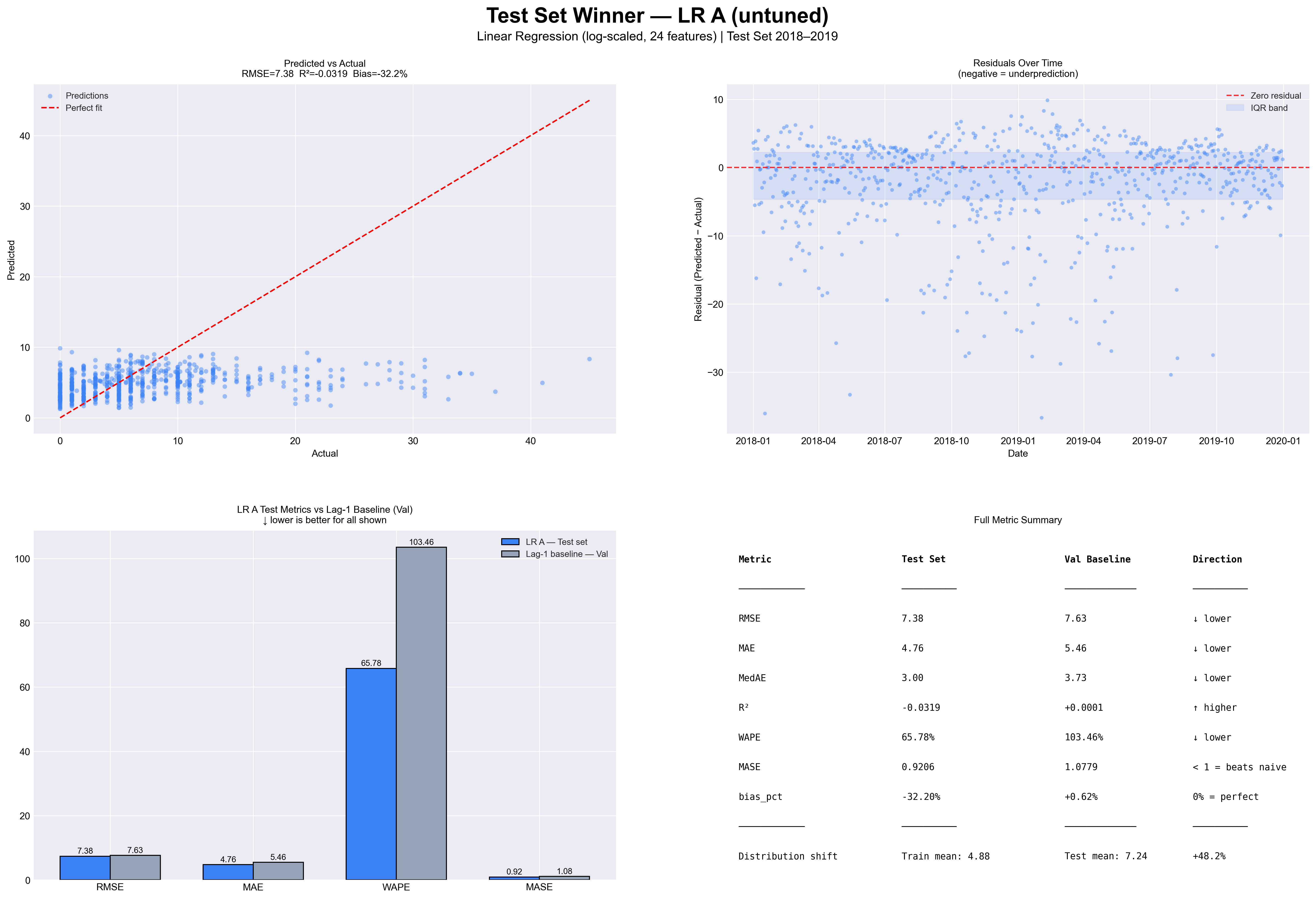
Everything above was validated on 2017 data. The real test came from 2018–2019, and it exposed something none of the validation-set results had shown: demand had shifted up by 48% between the training years and the test years. The test set's average was 7.24 units versus 4.88 in training; its 90th percentile was 16 versus 12; its maximum was 45 versus a training maximum of 36.

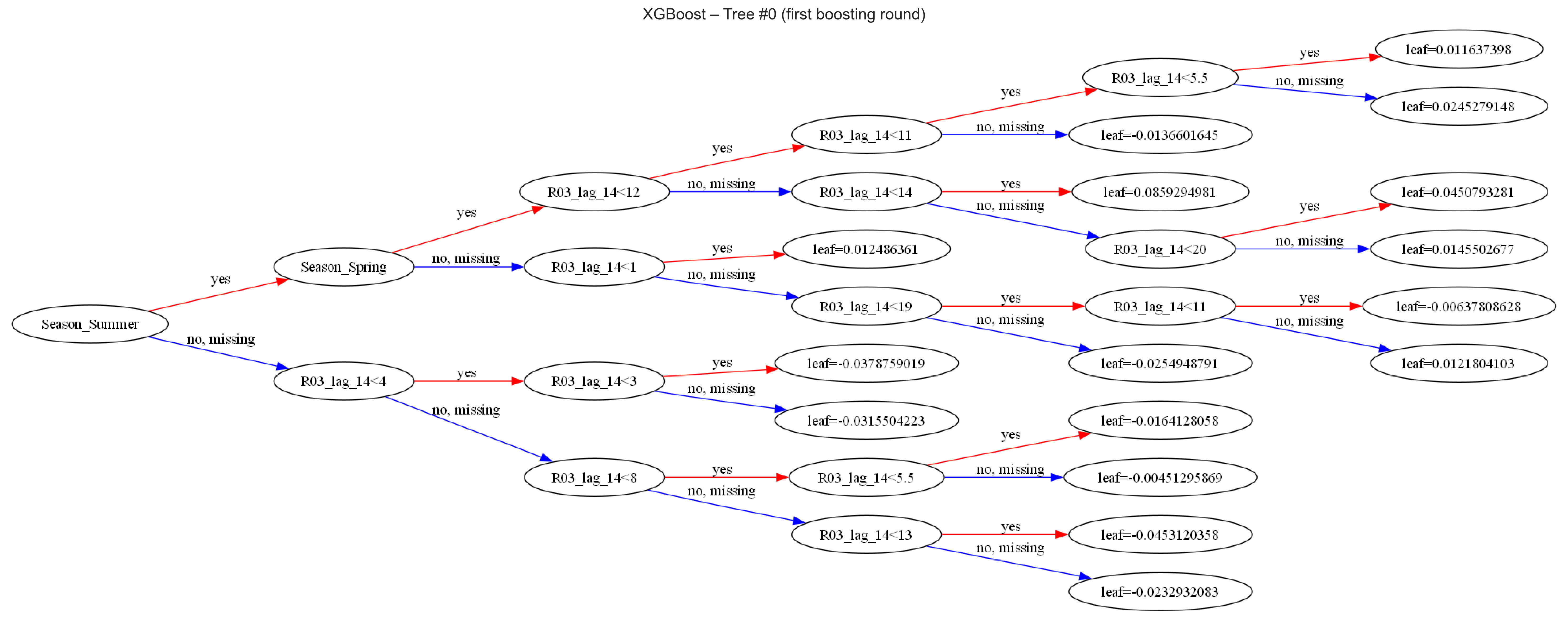
Tree-based models cannot extrapolate. A random forest, XGBoost, or LightGBM model predicts by averaging the training samples that land in the same leaf, so the highest possible prediction any of them can make is capped by the highest value they saw during training. When a 2019 winter week arrived with real demand north of 40, every tree model hit that ceiling and predicted low. Linear regression has no such ceiling; its coefficients define a hyperplane that keeps extending in whatever direction the data points. Combined with the log transformation, which makes the model's predictions scale multiplicatively rather than additively, linear regression was the only model architecturally capable of following the shift upward. Prophet failed even more dramatically (bias of 44% to 50%) for a related reason: it had fit a relatively flat trend line to 2014–2017 and simply extrapolated that flat trend forward, missing the level shift entirely.

The winning model, linear regression trained on log-scaled, 24 engineered features, posted a test-set MAE of 4.76 units and WAPE of 65.78%, not spectacular in absolute terms, but the best of the field, and for a legible, explainable reason rather than a black-box one.

What I'd take into a real deployment

A few honest caveats, because a forecasting model this far from "production-ready" deserves them:

• WAPE of ~66% is well above the ~35% benchmark typically expected in pharmaceutical retail forecasting. This model tells a clear methodological story; it isn't yet something I'd hand to a procurement team.
• The dataset itself has real limitations: a single pharmacy, no external variables (weather, flu severity, drug pricing), and a six-year window that ends before COVID,19 reshaped pharmacy demand entirely.
• The most valuable finding wasn't a model; it was a mismatch diagnosis. Knowing why the complex models failed (extrapolation limits, distributional shift) is more transferable to a real production system than any single R03 forecast is.

If I extended this, the two things I'd prioritize are external regressors (flu surveillance data, weather) and season-specific models, since the EDA made it clear that winter and summer R03 demand are close to two different problems wearing the same drug code.

This project uses the Wellness Pharmacy Sales Analysis dataset from Kaggle. Full notebook and code on Google Drive , or try the live predictor to see the winning model's forecasts against real 2018–2019 sales data it never trained on.